New in version 1.3: test.py has been created and thus, a new requirement on third-software is posted: NumPy and SciPy.
New in version 1.2: Command-line arguments parsed with argparse
New in version 1.1: report.py accepts a new collection of variables
New in version 1.1: score.py accepts now a new command-line argument --time
New in version 1.1: Welcome tscore.py!
IPCReport
While the design and implementation of the package IPCData (see IPCData) followed much the ideas that were already developed at the Sixth International Planning Competition in 2008, this package is brand new. It is mainly devoted to provide some simple (yet hopefully useful) mechanisms to access the data generated during the IPC or, alternatively, during a number of experiments.
The IPCReport package consists mainly of three different Python modules: report.py, score.py and tscore.py. While the first is intended to inspect the data generated by the invokeplanner.py module (see invokeplanner.py), the second and third have been developed to provide a consistent way to compute score tables and serves to compare the performance of a selected subset of planners in a selected subset of domains.
All these modules have been developed with Python 2.x
Dependencies
The modules described in this chapter have a number of dependencies with third-party software that have to be installed prior to the installation and usage of IPCReport:
pyExcelerator: This package provides an easy-to-use and clean interface to the generation of Excel worksheets with a number of nice features including colors, splitters, etc.
Instructions for downloading and installing the package are given here
numPy and SciPy: NumPy is, according to its authors, the fundamental package for scientific computing with Python. The SciPy library depends on NumPy, which provides convenient and fast N-dimensional array manipulation for different purposes.
Instructions to install these packages are given here
Finally, PrettyTable is used also. However, since it consists of a single module (i.e., no __init__ file is given), it is provided within the package IPCReport by default.
In what follows, it is assumed that the reader has already checked out to her local computer the scripts located at:
svn://svn@pleiades.plg.inf.uc3m.es/ipc2011/data/scripts/pycentral/IPCReport
Command-line arguments
All the modules in this package adhere to a consistent naming of the flags they acknowledge. This section describes this convention.
As a general rule all programs honour, at least, the following three flags:
-h, --help provide a brief description of the main purpose of the script and presents all the available flags -q, --quiet only prints the requested data -V, --version shows the current version of the script along with the head svn release that affects it and the building date
All the modules in package IPCReport can process data either from a results tree directory (see The results directory) or a summary —also known as snapshot, see Snapshots. While they cannot be specified simultaneously, one has to be provided with one of the following command-line arguments:
-d, --directory specifies the directory to explore. Their contents have to be consistent with the structure of the results directory, see The results directory -s, --summary instructs the script to retrieve the data contained in the binary file specified. For more information see Snapshots
On the other hand, all modules provide simple means to filter data by planner, domain and problem. In all cases, the given command-line argument receives a regular expression and only one:
-P, --planner only planners meeting the specified regexp are considered. All by default -D, --domain only domains meeting the specified regexp are considered. All by default -I, --problem only problem ids meeting the specified regexp are examined. All by default
The output of every module consists always of a table (with different sorts of data, according to the purpose of the module) that can be generated in different formats and can be given arbitrary names:
-n, --name name of the output table. In some cases, the name can acknowledge placeholders -y, --style sets the table type. At least, table, octave, html, excel and wiki are honoured by all modules. Exceptionally, score.py also welcomes latex
Most of these parameters accept a single value. However, some directives can be specified an arbitrary number of times. For example, one might want to examine the contents of the variables solved and oksolved with report.py. Instead of writing --variable solved --variable oksolved, it is possible to abbreviate it as --variable solved oksolved. Other directives that accept an arbitrary number of arguments are: --ascending and --descending
report.py
invokeplanner.py generates a particular tree structure that starts at the directory results/ in the same directory specified with the command-line option --directory. All modules of the package IPCReport are able to process the data in a results directory. However, this might result in large waiting times. To speed up the process, summaries (alternatively known also as snapshots) are provided.
While there is no need to be aware of the particular arrangement of the results directory structure it is described here succintly for the sake of completeness. Also, a gentle introduction to snapshots is provided immediately after. Most readers can safely skip the first two subsections and go directly to the next subsection that explains how to inspect data, Inspecting data.
The results directory
The contents of the results/ directory are sketched below:
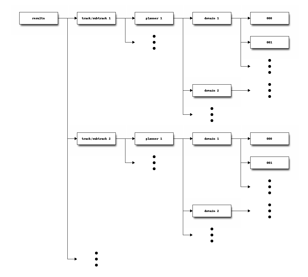
Therefore, the particular results of executing planner P in domain D in a particular track/subtrack are all stored in a number of directories 000/, 001/, ... To examine the results of one execution it is enough to examine the contents of that particular directory. Recall that these directories contain the problems and domains stored in the svn repository that result after sorting the names of domains (if more than one) and problems in lexicographical order —according to the cases single and multi, see builddomain.py.
In particular, the contents of the results directory of the Seventh International Planning Competition can be accessed in:
svn://svn@pleiades.plg.inf.uc3m.es/ipc2011/results
This repository contains three subdirectories:
logs/
This directory contains the execution log files that were generated by the script invokeplanner.py and also the standard output generated by the script itself. The first one refers to the logfile generated with the directive –logfile, and the second one is just the standard nohup.out output that results when running a process in background that is explicitly requested to do not be a child of the current shell process —explicitly requested with the /usr/bin/nohup command that automatically records the standard output to the file nohup.out.
For the sake of clarity, a chunk of the output of the log file specified with --logfile is shown here that shows the result of running all planners in the seq-opt competition with the sokoban domain:
[2011-03-30 12:55:49,375] [       plg@tau] [invoke_planner::show_switches] INFO

-----------------------------------------------------------------------------
 * Track     : 'seq'
 * Subtrack  : 'opt'
 * Planner   :  ['*']
 * Domain    :  ['sokoban']

 * Directory :  /home/plg/seq-opt-sokoban
 * Bookmark  :  svn+ssh://svn@korf.plg.inf.uc3m.es/ipc2011

 * Timeout   :  1800 seconds
 * Memory    :  6442450944 bytes
 -----------------------------------------------------------------------------

[2011-03-30 12:55:49,376] [       plg@tau] [invoke_planner::setup] INFO
  Building planner ...
[2011-03-30 12:55:50,209] [       plg@tau] [co_and_build] INFO
         Checking out bjolp in '/home/plg/seq-opt-sokoban/bjolp'
[2011-03-30 12:55:51,403] [       plg@tau] [buildplanner:co_and_build] INFO
         Building bjolp
[2011-03-30 12:59:15,735] [       plg@tau] [co_and_build] INFO
         Checking out cpt4 in '/home/plg/seq-opt-sokoban/cpt4'
[2011-03-30 12:59:21,068] [       plg@tau] [buildplanner:co_and_build] INFO
         Building cpt4

...

[2011-03-30 13:36:52,066] [       plg@tau] [invoke_planner::setup] INFO
  Building domain ...
[2011-03-30 13:36:52,735] [       plg@tau] [build_domain] INFO
         Building domain sokoban in '/home/plg/seq-opt-sokoban/sokoban'
[2011-03-30 13:37:01,694] [       plg@tau] [invoke_planner::setup] INFO
  Building workingdir /home/plg/seq-opt-sokoban/_bjolp.sokoban.000 ...
[2011-03-30 13:37:07,015] [       plg@tau] [invoke_planner::collect] INFO
  Collecting results in /home/plg/seq-opt-sokoban/_bjolp.sokoban.000 ...
[2011-03-30 13:37:07,064] [       plg@tau] [invoke_planner::setup] INFO
  Building workingdir /home/plg/seq-opt-sokoban/_bjolp.sokoban.001 ...

...

[2011-03-31 01:47:46,860] [       plg@tau] [invoke_planner::show_stats] INFO

 * Overall running time (seconds):
+------------------+---------------+---------------+
| *                |    sokoban    |     total     |
+------------------+---------------+---------------+
| bjolp            | 1078.88212848 | 1078.88212848 |
| cpt4             | 12922.8750858 | 12922.8750858 |
| fd-autotune      | 887.525495529 | 887.525495529 |
| fdss-1           |  616.94525528 |  616.94525528 |
| fdss-2           | 611.941836357 | 611.941836357 |
| forkinit         | 3423.95640659 | 3423.95640659 |
| gamer            | 17898.9191561 | 17898.9191561 |
| iforkinit        | 216.029652119 | 216.029652119 |
| lmcut            | 878.142556906 | 878.142556906 |
| lmfork           | 4155.72897196 | 4155.72897196 |
| merge-and-shrink | 611.936996937 | 611.936996937 |
| selmax           |  456.77576685 |  456.77576685 |
| total            | 43759.6593089 |               |
+------------------+---------------+---------------+

[2011-03-31 01:47:46,861] [       plg@tau] [invoke_planner::show_stats] INFO

 * Overall memory (Mbytes):
+------------------+---------------+---------------+
| *                |    sokoban    |     total     |
+------------------+---------------+---------------+
| bjolp            | 11903.9882812 | 11903.9882812 |
| cpt4             |  740.85546875 |  740.85546875 |
| fd-autotune      |  714.7890625  |  714.7890625  |
| fdss-1           |   10267.1875  |   10267.1875  |
| fdss-2           | 11388.7304688 | 11388.7304688 |
| forkinit         |  430.98046875 |  430.98046875 |
| gamer            | 63276.8867188 | 63276.8867188 |
| iforkinit        |   366.71875   |   366.71875   |
| lmcut            |  703.5390625  |  703.5390625  |
| lmfork           |  450.95703125 |  450.95703125 |
| merge-and-shrink | 11436.7890625 | 11436.7890625 |
| selmax           | 1637.82421875 | 1637.82421875 |
| total            | 113319.246094 |               |
+------------------+---------------+---------------+

[2011-03-31 01:47:46,862] [       plg@tau] [invoke_planner::show_stats] INFO

 * Number of solved instances:
+------------------+---------+-------+
| *                | sokoban | total |
+------------------+---------+-------+
| bjolp            |    20   |   20  |
| cpt4             |    1    |   1   |
| fd-autotune      |    20   |   20  |
| fdss-1           |    20   |   20  |
| fdss-2           |    20   |   20  |
| forkinit         |    19   |   19  |
| gamer            |    19   |   19  |
| iforkinit        |    20   |   20  |
| lmcut            |    20   |   20  |
| lmfork           |    19   |   19  |
| merge-and-shrink |    20   |   20  |
| selmax           |    20   |   20  |
| total            |   218   |       |
+------------------+---------+-------+

[2011-03-31 01:47:46,863] [       plg@tau] [invoke_planner::show_stats] INFO

 * Number of overall solutions generated:
+------------------+---------+-------+
| *                | sokoban | total |
+------------------+---------+-------+
| bjolp            |    20   |   20  |
| cpt4             |    1    |   1   |
| fd-autotune      |    20   |   20  |
| fdss-1           |    20   |   20  |
| fdss-2           |    20   |   20  |
| forkinit         |    19   |   19  |
| gamer            |    19   |   19  |
| iforkinit        |    20   |   20  |
| lmcut            |    20   |   20  |
| lmfork           |    19   |   19  |
| merge-and-shrink |    20   |   20  |
| selmax           |    20   |   20  |
| total            |   218   |       |
+------------------+---------+-------+
The dump shown above is divided in four sections: the first one shows some administrative information with the current version of the script along with a description of all the parameters given to it. Next, various INFO messages are issued to show what planners have been checked out from the svn repository and the exact times when they were compiled; the third part shows the testsets built; finally, a human-readable output is shown with some statistics about the overall performance of all planners.
On the other hand, the output of the nohup command is shown below:
Revision: 115
Date: 2011-03-27 16:08:59 +0200 (Sun, 27 Mar 2011)

./invokeplanner.py 1.0
There is no particular arrangement for the contents of the logs directory though the most usual is to have first a number of subdirectories sorted by track and subtrack. Beneath these directories different folders exist, each referring to a particular set of experiments. For example, a directory named acoplan means that it contains the output of running the planner acoplan with all domains. A subdirectory named barman shall be expected to contain the results of all planners when facing that particular domain, and so on.
raw/
This directory contains the tree structure that results after merging the directory results/ of all the experiments performed so far in all tracks.
However, none of these directories contain solutions validated by the Automatic Validation Tool VAL
val/
This directory follows the same structure than the directory raw/ but it contains only the minimum number of files that are necessary for validating each solution —if any was generated.
The script validate.py was later run on this directory, leaving a validation log file at each terminal directory with the result of the validation process. For more details, the interested reader is referred to validate.py
Therefore, from the previous descriptions it follows that all the results of the Seventh International Planning Competition are available in two different formats: either raw or validated. Unfortunately, processing these directories takes usually a long time. To speed it up snapshots are provided.
Snapshots
A snapshot (or alternatively, a summary) is just a binary file that contains the same relevant data stored in a results tree directory. Besides, it follows the same structure depicted there.
Snapshots provide a number of advantages:
Speed: handling a binary file is far faster than traversing a tree structure, visiting files and parsing their contents Size: besides, snapshots are usually smaller than a compressed file with the contents of a results directory so that they ease exchanging data among developers or the participants/organizers of an International Planning Competition
Snapshots are just created by instructing report.py to write the result of a query in a file specified with the directive --summarize, i.e., snapshots contain the results that were processed from a particular directory or another snapshot. In the first case, the tree that contains the data to inspect is specified with the directive --directory whereas a snapshot can be specified with the flag --summary —see Command-line arguments.
While they contain all the necessary information to understand and analyze the performance of each planner in every single domain, they are not easy to process manually. Instead, a dedicated module is devoted to this goal: report.py
Inspecting data
This section describes all the command-line arguments accepted by report.py. For a thorough discussion of the command-line arguments see Command-line arguments. Besides, the data retrieved with the script described here can be directly given to test.py (see test.py) to perform various sorts of statistical tests.
The report.py scripts accepts trees as the one described in subsection The results directory with the option --directory. Besides, it can also accept a binary file with the same contents, termed here as summaries or snapshots (see section Snapshots) with the directive --summary. In the following we will refer both to the snapshots and the results tree directories as the origin.
The specified origin automatically sets the level of the query. If it refers to a directory that looks like track-n-subtrack-m (such as seq-sat), the query refers to the whole track/subtrack; if the origin is relative to a directory such as planner-p (such as cbp), the queries are referred only to that particular planner in the track/subtrack that contains it; if the origin points deeper to domain-d (e.g., tidybot) then all queries are relative to the combination of planner and domain that are defined within that particular track/subtrack. Finally, specifying an origin with a particular problem restricts all queries to that particular problem. However, the level set by default by a particular origin can be altered with --level. Both snapshots and results tree directories are arranged as explained in The results directory. Therefore, the only legal levels are: planner, domain and problem and in exactly that order. Obviously, the level cannot be pushed up (e.g., involving other planners when specifying a domain) but it can be refined further by specifying any of the legal levels if and only if the origin is the same or above than the specified level.
Furthermore, queries can be refined by a number of arguments, as explained in Command-line arguments by providing one (and only one) regular expression to any of the following directives: --planner, --domain and/or --problem. They can be provided in any combination. For example, --planner lama --domain p --problem "0[01][02468]" retrieves information for the problems with an even identifier in those domains that start with p that where given to planners whose name starts with lama.
report.py acknowledges a number of variables whose values are returned after inspecting the corresponding origin. The list of available variables is listed if --variables is specified in the command line —for a thorough introduction to the variables acknowledged by report.py the reader is referred to Reporting variables. Variables are specified with the directive --variable. There is no need to use the directive more than once unless the specification of different variables happen in different locations of the command-line. For example, to access vars var1, var2, var3, ... the following suffices: --variable var1 var2 var3 .... The report will show the variables in the same order they have been specified so that the same results can be achieved with --variable var3 var2 var1 ... but in a different order.
For example, the number of problems in the sequential satisficing track of the Seventh International Planning Competition can be retrieved with the following command:
 $ ./report.py --directory /Volumes/Owl/Downloads/ipc2011/results/val/seq-sat
   --variable numprobs --summarize seq-sat.snapshot

 Revision: 282
 Date: 2011-07-04 10:48:49 +0200 (Mon, 04 Jul 2011)

 ./report.py 1.0

 -----------------------------------------------------------------------------
 * directory      : /Volumes/Owl/Downloads/ipc2011/results/val/seq-sat
 * snapshot       : /Users/clinares/lab/ipc2011-data/scripts/pycentral/IPCReport/seq-sat.snapshot
 * name           : report
 * level          : None
 * planner        : .*
 * domain         : .*
 * problem        : .*
 * variables      : ['numprobs']
 * unroll         : False
 * sorting        : []
 * style          : table
 -----------------------------------------------------------------------------

 name: report
+----------+
| numprobs |
+----------+
|   7560   |
+----------+
 legend:
   numprobs: total number of problems [elaborated data]

 created by IPCrun 1.0 (Revision: 283), Thu Jul 21 13:42:08 2011
Note that the preceding command creates also a summary with all the data that results from processing all the tree structure rooted at the particular location given /Volumes/Owl/Downloads/ipc2011/results/val/seq-sat
The same query can be refined further requesting the number of problems by planner just by altering the level as follows:
 $ ./report.py --summary seq-sat.snapshot --variable numprobs --level planner

 Revision: 282
 Date: 2011-07-04 10:48:49 +0200 (Mon, 04 Jul 2011)

 ./report.py 1.0

 -----------------------------------------------------------------------------
 * summary        : /Users/clinares/lab/ipc2011-data/scripts/pycentral/IPCReport/seq-sat.snapshot
 * snapshot       :
 * name           : report
 * level          : planner
 * planner        : .*
 * domain         : .*
 * problem        : .*
 * variables      : ['numprobs']
 * unroll         : False
 * sorting        : []
 * style          : table
 -----------------------------------------------------------------------------

 name: report
+---------------+----------+
|    planner    | numprobs |
+---------------+----------+
|    acoplan    |   280    |
|    acoplan2   |   280    |
|     arvand    |   280    |
|      brt      |   280    |
|      cbp      |   280    |
|      cbp2     |   280    |
|      cpt4     |   280    |
|   dae_yahsp   |   280    |
| fd-autotune-1 |   280    |
| fd-autotune-2 |   280    |
|     fdss-1    |   280    |
|     fdss-2    |   280    |
|  forkuniform  |   280    |
|   lama-2008   |   280    |
|   lama-2011   |   280    |
|     lamar     |   280    |
|     lprpgp    |   280    |
|   madagascar  |   280    |
|  madagascar-p |   280    |
|     popf2     |   280    |
|     probe     |   280    |
|    randward   |   280    |
|     roamer    |   280    |
|  satplanlm-c  |   280    |
|    sharaabi   |   280    |
|     yahsp2    |   280    |
|   yahsp2-mt   |   280    |
+---------------+----------+
 legend:
   planner [key]
   numprobs: total number of problems [elaborated data]

 created by IPCrun 1.0 (Revision: 283), Thu Jul 21 13:43:36 2011
Note that because a snapshot was created in the first query, it is now feasible to use it instead of directly accessing the tree structure. This procedure actually saves a lot of time and goes far faster.
Of course, variables can be combined. For example, the following command returns the number of problems, the number of solved tasks (but not validated) and the number of problems where the winners of the Sixth International Planning Competition (LAMA 2008) and the Seventh International Planning Competition (LAMA 2011) failed:
 $ /report.py --summary seq-sat.snapshot --planner 'lama.*20.*' --level planner
   --variable numprobs numsolved numfails --quiet

 name: report
+-----------+----------+-----------+----------+
|  planner  | numprobs | numsolved | numfails |
+-----------+----------+-----------+----------+
| lama-2008 |   280    |    188    |    92    |
| lama-2011 |   280    |    250    |    30    |
+-----------+----------+-----------+----------+
 legend:
   planner [key]
   numprobs: total number of problems [elaborated data]
   numsolved: number of solved problems (independently of the solution files generated) [elaborated data]
   numfails: total number of fails [elaborated data]

 created by IPCrun 1.0 (Revision: 283), Thu Jul 21 13:51:06 2011
In this case, because the directive --quiet was given, all the headers were removed from the output.
Moreover, the results can be sorted either in ascending or descending order of any combination of variables thanks to the flags --ascending and --descending. These variables shall be given along with one of the variables specified in the query and/or any of the legal levels: planner, domain and/or problem. For example, the following command shows the number of problems successfully solved and the number of plan solution files generated by all planners in the sequential satisficing track. It then sorts the output giving preference to the planners that solved more tasks and, in case of a tie (note the case of planners probe and fdss-2 both with 233 tasks solved), it ranks first those that generated more solution files:
$ ./report.py --summary seq-sat.snapshot --variable oknumsolved oksumnumsols
  --level planner --quiet --descending oknumsolved --descending oksumnumsols
 name: report
+---------------+-------------+--------------+
|    planner    | oknumsolved | oksumnumsols |
+---------------+-------------+--------------+
|   lama-2011   |     250     |     874      |
|     fdss-2    |     233     |     645      |
|     probe     |     233     |     460      |
|     fdss-1    |     232     |     828      |
| fd-autotune-1 |     223     |     557      |
|     roamer    |     213     |     779      |
|  forkuniform  |     207     |     589      |
|     lamar     |     195     |     764      |
| fd-autotune-2 |     193     |     516      |
|     arvand    |     190     |     1813     |
|   lama-2008   |     188     |     743      |
|    randward   |     184     |     689      |
|      brt      |     157     |     499      |
|     yahsp2    |     138     |     246      |
|   yahsp2-mt   |     137     |     423      |
|      cbp2     |     135     |     834      |
|      cbp      |     123     |     788      |
|   dae_yahsp   |     120     |     963      |
|     lprpgp    |     118     |     236      |
|  madagascar-p |      88     |      88      |
|     popf2     |      81     |     100      |
|   madagascar  |      67     |      67      |
|      cpt4     |      52     |      52      |
|    sharaabi   |      33     |      33      |
|  satplanlm-c  |      32     |      32      |
|    acoplan    |      20     |      80      |
|    acoplan2   |      20     |      70      |
+---------------+-------------+--------------+
 legend:
   planner [key]
   oknumsolved: number of *successfully* solved problems (independently of the solution files generated)
                [elaborated data]
   oksumnumsols: sum of the total number of *successful* solution files generated [elaborated data]

 created by IPCrun 1.0 (Revision: 283), Thu Jul 21 14:09:09 2011
Another very interesting flag is --unroll. This flag correlates the values of an arbitrary number of variables —usually two. If the values of all variables are lists then --unroll creates as many rows in the resulting table as elements in the shortest list. For example, to show how the quality of the solutions generated by arvand in problem 011 of the domain openstacks improved over time:
$ /report.py --summary seq-sat.snapshot --quiet
  --planner 'arvand' --level problem --domain 'openstacks' --problem '011'
  --variable timesols values --unroll

 name: report
+---------+------------+---------+----------+--------+
| planner |   domain   | problem | timesols | values |
+---------+------------+---------+----------+--------+
|  arvand | openstacks |   011   |    19    | 126.0  |
|  arvand | openstacks |   011   |    27    | 125.0  |
|  arvand | openstacks |   011   |    63    | 123.0  |
|  arvand | openstacks |   011   |   173    | 122.0  |
|  arvand | openstacks |   011   |   181    | 121.0  |
|  arvand | openstacks |   011   |   257    | 120.0  |
|  arvand | openstacks |   011   |   266    | 118.0  |
|  arvand | openstacks |   011   |   375    | 116.0  |
|  arvand | openstacks |   011   |   425    | 115.0  |
|  arvand | openstacks |   011   |   478    | 113.0  |
|  arvand | openstacks |   011   |   589    | 112.0  |
|  arvand | openstacks |   011   |   755    | 111.0  |
|  arvand | openstacks |   011   |   876    | 110.0  |
|  arvand | openstacks |   011   |   931    | 109.0  |
+---------+------------+---------+----------+--------+
 legend:
   planner [key]
   domain [key]
   problem [key]
   timesols: elapsed time when each solution was generated (in seconds) [raw data]
   values: final values returned by VAL, one per each *valid* solution file [raw data]

 created by IPCrun 1.0 (Revision: 283), Thu Jul 21 14:22:04 2011
Should --unroll not have been given, the report would have just issued a single line with one list per variable, which is not the desired effect.
Because report.py acknowledges a number of output formats with the flag --style, --unroll is very useful for creating figures. The available styles are table, octave, html, excel and wiki. The first is used by default. octave shows the same information but in the format of GNU Octave which can be read also by gnuplot. html and wiki are markup languages to show the same data either in html pages or in the wiki format recognized by MoinMoin. Finally, excel creates a file named report.xls with the result of the query.
The last directive that affects the output is --name. It can be used to give the resulting table an arbitrary name.
score.py
This section describes all the command-line arguments accepted by score.py. For a thorough discussion of the command-line arguments see Command-line arguments.
This script automatically generates score tables for a selected subset of domains, planners and problems. As in the case of report.py (see report.py), this script receives either a results tree (as the one depicted in The results directory) or a snapshot —as described in Snapshots. Let origin denote both a result directory and a snapshot or summary —note that score.py does not generate any snapshots and that only report.py can do it, for more information refer to the directive --summarize in Inspecting data. The origin shall refer always to a whole track-subtrack. This is, it is not valid to specify either a directory or a snapshot that points to a planner, domain or problem.
The collection of planners, domains and problems to consider can be refined further with regular expresions with --planner, --domain and --problem.
If the directive --time is given, then all measurements are relative to the time interval [0, time] (where time is the value given to --time in seconds). If none is specified, then all results are used. This allows drawing conclusions for different time horizons, others than that used in the experimentation —see the usage of the directive --timeout in invokeplanner.py.
score.py acknowledges up to six different metrics. All of them are described if the directive --metrics is given:
quality: This is the official metric of both the Sixth and Seventh International Planning Competitions. It computes for each task a score which equals
where
is the quality of the best plan found for this particular task and
stands for the quality of the plan produced by this planner.
solutions: It gives one point to every planner that solves the current task and zero otherwise.
time0: Computes the score of a planner for a given task as the quotient
where
is the minimum time required by any planner to solve the same task and
is the time it took this particular planner to solve the same task.
All times below 1 second are considered to be exactly equal to 1 second. In other words, differences below one second are considered to be negligible.
time1: Computes the score of a planner for a given task as the quotient
where
All times below 1 second are considered to be exactly equal to 1 second. In other words, differences below one second are considered to be negligible.
time2: Computes the score of a planner for a given task as the quotient
where
qt: It computes for each planner and task a tuple
where
if and only if
and

All the scores are shown in the form of tables, one per domain that meet the regular expression given to --domain. Besides, if more than one domain is given, the script computes a final table called ranking with the sum of the scores of all the previous tables. Each table can be given a name with --name. This directive accepts placeholders which are symbolized with the dollar sign $. In particular, there are five recognized variables: $track, $subtrack, $domain, $date and $time which are substituted with the particular track, subtrack, domain, current date and time. The default value of this variable is $track-$subtrack: $domain ($date) [1].
For example, the following command:
$ /score.py --summary seq-opt.results.snapshot
            --planner 'f' --domain 'sokoban|parcprinter' --time 10
will output the score tables for those planners of the sequential optimization track that start with the letter f in the domains sokoban and parcprinter taking into account only the results that were produced in the first 10 seconds —though the specified snapshot contains the results of running the planners up to 1800 seconds. The metric used is the default one quality and the output (discussed below) is just shown as ASCII tables:
seq-opt: parcprinter (Mon Dec 19 23:35:01 2011)
+-------+-------------+--------+--------+----------+------------+
|  no.  | fd-autotune | fdss-1 | fdss-2 | forkinit |    best    |
+-------+-------------+--------+--------+----------+------------+
|  000  |     1.00    |  1.00  |  1.00  |   1.00   | 375821.00  |
|  001  |     1.00    |  1.00  |  1.00  |   1.00   | 438047.00  |
|  002  |     1.00    |  1.00  |  1.00  |   1.00   | 510256.00  |
|  003  |     1.00    |  1.00  |  1.00  |   ---    | 876094.00  |
|  004  |     1.00    |  1.00  |  1.00  |   1.00   | 519232.00  |
|  005  |     ---     |  ---   |  ---   |   ---    |    ---     |
|  006  |     1.00    |  ---   |  ---   |   ---    | 1145132.00 |
|  007  |     1.00    |  1.00  |  1.00  |   1.00   | 751642.00  |
|  008  |     1.00    |  1.00  |  1.00  |   1.00   | 693064.00  |
|  009  |     ---     |  ---   |  ---   |   ---    |    ---     |
|  010  |     1.00    |  ---   |  ---   |   ---    | 1216462.00 |
|  011  |     ---     |  ---   |  ---   |   ---    |    ---     |
|  012  |     ---     |  ---   |  ---   |   ---    |    ---     |
|  013  |     ---     |  ---   |  ---   |   ---    |    ---     |
|  014  |     ---     |  ---   |  ---   |   ---    |    ---     |
|  015  |     ---     |  ---   |  ---   |   ---    |    ---     |
|  016  |     ---     |  ---   |  ---   |   ---    |    ---     |
|  017  |     ---     |  ---   |  ---   |   ---    |    ---     |
|  018  |     ---     |  ---   |  ---   |   ---    |    ---     |
|  019  |     1.00    |  ---   |  ---   |   ---    | 1270874.00 |
| total |    10.00    |  7.00  |  7.00  |   6.00   |            |
+-------+-------------+--------+--------+----------+------------+

 ---: unsolved
  X : invalid

 created by IPCrun 1.2 (Revision: 295), Mon Dec 19 23:35:01 2011


seq-opt: sokoban (Mon Dec 19 23:35:01 2011)
+-------+-------------+--------+--------+----------+-------+
|  no.  | fd-autotune | fdss-1 | fdss-2 | forkinit |  best |
+-------+-------------+--------+--------+----------+-------+
|  000  |     1.00    |  1.00  |  1.00  |   1.00   |  9.00 |
|  001  |     1.00    |  1.00  |  1.00  |   1.00   | 37.00 |
|  002  |     1.00    |  1.00  |  1.00  |   1.00   | 29.00 |
|  003  |     1.00    |  1.00  |  1.00  |   1.00   | 29.00 |
|  004  |     ---     |  1.00  |  1.00  |   ---    | 50.00 |
|  005  |     ---     |  1.00  |  1.00  |   ---    | 35.00 |
|  006  |     1.00    |  1.00  |  1.00  |   1.00   | 30.00 |
|  007  |     1.00    |  1.00  |  1.00  |   1.00   | 19.00 |
|  008  |     1.00    |  1.00  |  1.00  |   1.00   | 15.00 |
|  009  |     1.00    |  1.00  |  1.00  |   1.00   |  8.00 |
|  010  |     1.00    |  1.00  |  1.00  |   1.00   | 20.00 |
|  011  |     1.00    |  1.00  |  1.00  |   1.00   |  2.00 |
|  012  |     ---     |  ---   |  ---   |   ---    |  ---  |
|  013  |     1.00    |  ---   |  ---   |   1.00   | 32.00 |
|  014  |     ---     |  ---   |  ---   |   ---    |  ---  |
|  015  |     ---     |  ---   |  ---   |   ---    |  ---  |
|  016  |     ---     |  ---   |  ---   |   ---    |  ---  |
|  017  |     1.00    |  1.00  |  1.00  |   ---    | 10.00 |
|  018  |     ---     |  ---   |  ---   |   ---    |  ---  |
|  019  |     ---     |  ---   |  ---   |   ---    |  ---  |
| total |    12.00    | 13.00  | 13.00  |  11.00   |       |
+-------+-------------+--------+--------+----------+-------+

 ---: unsolved
  X : invalid

 created by IPCrun 1.2 (Revision: 295), Mon Dec 19 23:35:01 2011


seq-opt: ranking (Mon Dec 19 23:35:01 2011)
+-------------+---------+-------------+-------+
|   planner   | sokoban | parcprinter | total |
+-------------+---------+-------------+-------+
| fd-autotune |  12.00  |    10.00    | 22.00 |
|    fdss-1   |  13.00  |     7.00    | 20.00 |
|    fdss-2   |  13.00  |     7.00    | 20.00 |
|   forkinit  |  11.00  |     6.00    | 17.00 |
|    total    |  49.00  |    30.00    |       |
+-------------+---------+-------------+-------+

 ---: unsolved
  X : invalid

 created by IPCrun 1.2 (Revision: 295), Mon Dec 19 23:35:01 2011
Finally, score.py can produce the output in a variety of formats. It recognizes at least the same ones described in Inspecting data and, additionally, latex. If used, it creates a LaTeX file called matrix.tex. Each page is divided in two halves: the upper contains the table whereas the lower half shows up a matrix of color codes with the following meanings:
Red boxes: invalid entry. The planner generated a solution but it was considered invalid by the Automatic Validation Tool VAL Yellow boxes: empty solution. The planner never found a solution for this task. Gray boxes: solved tasks. It uses gray levels to mean scores. The darker the better.
Since the resulting LaTeX file uses ps-tricks it cannot be processed directly with pdflatex. Instead, a makefile is given in the same directory where this package resides. To produce the corresponding pdf file just type:
$ make filename.pdf
where filename stands for the name of the LaTeX file —matrix in this case.
tscore.py
This script behaves much the same like score.py but with a key difference. While it acknowledges the same directives than the previous script (though no LaTeX output is supported), it just computes how the score of all planners evolve over time on all the selected domains.
These figures are computed taking for each planner the time when they generate a solution. This is, at each time instant, where at least one planner among those selected by the regular expression given in --planner found a solution to at least one problem in a particular domain, the score of all planners is computed. This process produces a curve that shows how the score of each planner evolved over time at precise time instants.
Since this computation can be costly (a matter of minutes in the larger tracks if direct access to the result directories is being performed instead of snapshots), the script also acknowledges a new flag --labels. This directive allows the user to specify a number of time points which are drawn from the original list of time instants at regular intervals —this implies that the final number of points drawn might not be exactly equal to the number requested by the user, though it will be always as close as possible.
For example, the following command computes how the score evolves over time for the six top ranked planners in the Seventh International Planning Competition (if more than one variant of the same planner ranked among these, the best is picked up) for the domain barman:
$ ./tscore.py --summary seq-sat.snapshot --metric quality
  --planner "lama-2011|fdss-1|fd-autotune-1|roamer|forkuniform|probe" --domain "barman"
  --style octave --quiet > salida.m
Now, if all matrices in the output file salida.m are removed but scores_barman, the following commands in gnuplot:
gnuplot> set xlabel "Time (seconds)"
gnuplot> set ylabel "Score"
gnuplot> set terminal png
gnuplot> set output "barman.png"
gnuplot> plot "salida.m" using 1:2 with linesp title "fd-autotune-1",
              "salida.m" using 1:3 with linesp title "fdss-1",
              "salida.m" using 1:4 with linesp title "forkuniform",
              "salida.m" using 1:5 with linesp title "lama-2011",
              "salida.m" using 1:6 with linesp title "probe",
              "salida.m" using 1:7 with linesp title "roamer"
produce the following output:
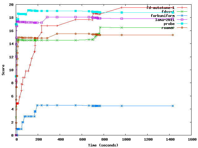
which can be used to draw a number of interesting conclusions.
Even if only one domain meets the regular expression specified with --domain this scripts shows up an overall ranking table at the end. This table takes the time instant where at least one planner solved one task in any of the domains specified. Besides, while the tables generated per domain list planners in alphabetical order, the overall ranking table shows them in decreasing order of total score.
test.py
In most cases, looking at the number of problems solved, their plan quality or other characteristics is not enough to judge whether one planner performs better than another. This problem is rather typical in many fields of Science (including Artificial Intelligence) and the usual approach consists of performing statistical tests. Since the module IPCReport already provides a facility to access data (see report.py), it is almost straightforward to provide another script to perform statistical tests over the same data. This is the target of test.py. This script uses report.py transparently to the user to retrieve data from a snapshot or summary (see Snapshots) or results tree directory (see The results directory) and perform the indicated statistical tests over the resulting series.
The script test.py implements four different statistical tests. Since parametrical statistical tests make questionnable assumptions about the distribution of data, and besides most series are more likely to be relatively short (e.g., in the seventh International Planning Competition there were 20 planning tasks per domain so that most series have n=20 samples which is regarded in some texts as being borderline between a small and large set) three of them are nonparametric. However, because of its popularity, a fourth one which is parametric is included as well:
Mann-Whitney U-test: It compares two samples that are independent, or not related. It assesses whether one of two samples of independent observations tends to have larger values than the other. The test automatically corrects for ties and by default uses a continuity correction. The reported p-value is for a one-tailed hypothesis, i.~e., when information about whether one sample have larger values than the other is provided. To get the two-tailed p-value (i.~e., when the null hypothesis is rejected if the test statistic is either too small or too large) the returned p-value has to be multiplied by two.
Wilcoxon signed rank test: In contraposition to the previous test, the Wilcoxon signed rank test is a two-tailed nonparametric statistical procedure for comparing two samples that are paired, or related. It tests the null hypothesis that both samples come from the same distribution.
This test has been extensively used in the analysis of previous International Planning Competitions, mostly in the third and fifth.
Binomial test: It is an exact test used with dichotomous data —that is, when each individual in the sample is classified in one of two categories such as success/failure. It provides statistical significance of deviations from a binomial distribution with p=0.5.
The use of this test in the context of Automated Planning was originally proposed by Hoffmann and Nebel to provide statistical significance of the differences in performance of their planner FF when using different combinations of enhancements
t-Test: It is the parametric equivalent test of the Wilcoxon signed rank test. This is a two-tailed test for the null hypothesis that two independent samples have identical average (expected) values
One restriction of all of these tests, however, is that they just compare two series of data. Other tests such as, the Kolmogorov-Smirnov one-sample test to determine if a data sample meets acceptable levels of normality or the Friedmann or the Kruskal-Wallis H-tests to compare three or more samples (either related or unrelated respectively), are not currently implemented. Instead, all these statistical tests perform pairwise comparisons of an arbitrary number of series and provide the p-value of each pair according to the selected statistical procedure. If the resulting p-value is less or equal than the critical value that corresponds to a particular level of risk α, the null hypothesis is rejected and the alternate or research hypothesis is accepted instead. Typical values of the level of risk are α=0.05, 0.01 and 0.001 which stand for a probability of 95%, 99% and 99.9% respectively that any observed statistical difference will be real and not due to chance.
This script retrieves data from report.py (see report.py) transparently to the user so that it acknowledges the same directives that can be used with exactly the same purpose but just one restriction: only one variable (with --variable) can be provided so that only single-valued series are allowed. Once report.py has been silently invoked it retrieves a unique table of data which is split in as many series as primary keys are present in the table by test.py. For example, the following query returns the number of problems apparently solved (i.e., that the planner claims that it solved) and those that are successfully solved (i.e., validated with VAL) in the woodworking domain by planners fdss-2, lmcut and gamer:
$ ./report.py --summary ./seq-opt.results.snapshot --variable solved oksolved
              --domain woodworking --planner 'fdss-2|lmcut|gamer'

  +---------+-------------+---------+--------+----------+
  | planner |    domain   | problem | solved | oksolved |
  +---------+-------------+---------+--------+----------+
  |  fdss-2 | woodworking |   000   |  True  |   True   |
  |  fdss-2 | woodworking |   001   |  True  |   True   |
  |  fdss-2 | woodworking |   002   |  True  |   True   |
  |  fdss-2 | woodworking |   003   |  True  |   True   |
  |  fdss-2 | woodworking |   004   |  True  |   True   |
  |  fdss-2 | woodworking |   005   |  True  |   True   |
  |  fdss-2 | woodworking |   006   |  True  |   True   |
  |  fdss-2 | woodworking |   007   |  True  |   True   |
  |  fdss-2 | woodworking |   008   |  True  |   True   |
  |  fdss-2 | woodworking |   009   |  True  |   True   |
  |  fdss-2 | woodworking |   010   | False  |  False   |
  |  fdss-2 | woodworking |   011   | False  |  False   |
  |  fdss-2 | woodworking |   012   | False  |  False   |
  |  fdss-2 | woodworking |   013   | False  |  False   |
  |  fdss-2 | woodworking |   014   |  True  |   True   |
  |  fdss-2 | woodworking |   015   | False  |  False   |
  |  fdss-2 | woodworking |   016   | False  |  False   |
  |  fdss-2 | woodworking |   017   | False  |  False   |
  |  fdss-2 | woodworking |   018   | False  |  False   |
  |  fdss-2 | woodworking |   019   | False  |  False   |
  |  gamer  | woodworking |   000   |  True  |   True   |
  |  gamer  | woodworking |   001   |  True  |   True   |
  |  gamer  | woodworking |   002   |  True  |   True   |
  |  gamer  | woodworking |   003   |  True  |   True   |
  |  gamer  | woodworking |   004   |  True  |   True   |
  |  gamer  | woodworking |   005   |  True  |   True   |
  |  gamer  | woodworking |   006   |  True  |   True   |
  |  gamer  | woodworking |   007   |  True  |   True   |
  |  gamer  | woodworking |   008   |  True  |   True   |
  |  gamer  | woodworking |   009   |  True  |   True   |
  |  gamer  | woodworking |   010   |  True  |   True   |
  |  gamer  | woodworking |   011   |  True  |   True   |
  |  gamer  | woodworking |   012   |  True  |   True   |
  |  gamer  | woodworking |   013   |  True  |   True   |
  |  gamer  | woodworking |   014   |  True  |   True   |
  |  gamer  | woodworking |   015   |  True  |   True   |
  |  gamer  | woodworking |   016   | False  |  False   |
  |  gamer  | woodworking |   017   | False  |  False   |
  |  gamer  | woodworking |   018   |  True  |   True   |
  |  gamer  | woodworking |   019   | False  |  False   |
  |  lmcut  | woodworking |   000   |  True  |   True   |
  |  lmcut  | woodworking |   001   |  True  |   True   |
  |  lmcut  | woodworking |   002   |  True  |   True   |
  |  lmcut  | woodworking |   003   |  True  |   True   |
  |  lmcut  | woodworking |   004   |  True  |   True   |
  |  lmcut  | woodworking |   005   |  True  |   True   |
  |  lmcut  | woodworking |   006   |  True  |   True   |
  |  lmcut  | woodworking |   007   |  True  |   True   |
  |  lmcut  | woodworking |   008   |  True  |   True   |
  |  lmcut  | woodworking |   009   |  True  |   True   |
  |  lmcut  | woodworking |   010   | False  |  False   |
  |  lmcut  | woodworking |   011   | False  |  False   |
  |  lmcut  | woodworking |   012   | False  |  False   |
  |  lmcut  | woodworking |   013   | False  |  False   |
  |  lmcut  | woodworking |   014   |  True  |   True   |
  |  lmcut  | woodworking |   015   |  True  |   True   |
  |  lmcut  | woodworking |   016   | False  |  False   |
  |  lmcut  | woodworking |   017   | False  |  False   |
  |  lmcut  | woodworking |   018   | False  |  False   |
  |  lmcut  | woodworking |   019   | False  |  False   |
  +---------+-------------+---------+--------+----------+
The primary key in this case is planner which is instatiated to fdss-2, gamer and lmcut. Therefore, test.py automatically creates three series with the values of a single variable for these keys —in the previous example solved was shown also to exemplify below how two variables can be used simultaneously with the directive --filter.
Observing the number of solved problems in this particular domain, it turns out that gamer seems to be the best (solving 17 problems) followed by lmcut (which solves 12) and fdss-2 which solves 11. However, performing a statistical test over these series will provide a more reliable impression of the relative performance of these planners. Since the data in these series are dichotomic (it only takes the values True and False) a Binomial test is performed to know whether one planner performs better than another. Initially, one can directly ask test.py to perform the statistical test just passing by the same parameters but with just one single variable of interest, oksolved along with the particular selection of the statistical test to perform with the option --test:
$ ./test.py --summary ./seq-opt.results.snapshot --variable oksolved
            --domain woodworking --planner 'fdss-2|lmcut|gamer' --test bt

   Revision
   Date

   ./test.py 1.3

   -----------------------------------------------------------------------------
   * snapshot       : ./seq-opt.results.snapshot
   * tests          : ['Binomial test']
   * name           : report
   * level          : None
   * planner        : fdss-2|lmcut|gamer
   * domain         : woodworking
   * problem        : .*
   * variable       : ['oksolved']
   * filter         : None
   * matcher        : all
   * noentry        : -1
   * unroll         : False
   * sorting        : []
   * style          : table
   -----------------------------------------------------------------------------


   name: report
  +--------+----------+-------+---------+
  |        |  fdss-2  | gamer |  lmcut  |
  +--------+----------+-------+---------+
  | fdss-2 |   ---    |  1.0  |   1.0   |
  | gamer  | 0.015625 |  ---  | 0.03125 |
  | lmcut  |   0.5    |  1.0  |   ---   |
  +--------+----------+-------+---------+
   Binomial test : Perform a binomial two-sided sign test. It computes the number n of times that the serie
   shown in the row behaves differently than the serie shown in the column. It returns the probability
   according to a binomial distribution with p=0.5 that the number of times that the serie shown in the row
   takes values larger than the serie shown in the column equals at least the number of times that this
   difference was observed.
   If this probability is less or equal than a given threshold, e.g., 0.01, 0.05 or 0.1, then reject
   the null hypothesis and assume that the serie shown in the column is significantly smaller

   created by IPCtest 1.3 (Revision: 312), Sun Jul 15 17:21:38 2012
It is possible to invoke test.py with the option --tests to get a full list of all the implemented statistical tests along with a description of their use and purpose. It is also feasible to request an arbitrary number of statistical tests passing them altogether after --test —as in --test wx mw which requests simultaneously the Wilcoxon Signed-rank test and Mann Whitney U test.
From the preceding figure, it seems that fdss-2 and lmcut perform better than gamer with a confidence level α=0.05 (i.e., with a probability equal to 95%). This result goes against the original intuition. The reason is that the Binomial test tests whether the planner in the colum has values smallers than the planner shown in the row. Since False is considered to be smaller than True in most computing languages (including Python) the results are clearly misleading. To correct the results it is neccessary to provide a larger value to those problems that were not solved.
Hence, the first step consists of filtering data. In this case, the variable of interest is solved (whether the planner provided at least one solution to a single planning task) which is filtered by oksolved —whether the plan found is valid or not. A filter (oksolved in the following example) sets the value of a particular sample to the constant NOENTRY if it is False and passes the value of the selected variable (solved) in case it is True. In other words, it filters the input data according to a secondary variable. The primary variable is selected with --variable (as in report.py), whereas the secondary variable is selected with --filter. However, filtering data poses a new question: When comparing two series, what to do with those entries in one serie whose value equals NOENTRY?
Sometimes it is desirable to compare only those entries from two series where both elements have been filtered —these are known as double hits. In other cases, it might be better to preserve those entries where only one serie has the value NOENTRY. The third alternative consists of comparing both series even if the same entry contains NOENTRY for both series. This selection can be performed with --matcher which accepts the values and, or and all to match two series as indicated before respectively:
and: It only accepts those entries where both series have values different than NOENTRY or: It rejects only those entries where both series have values equal to NOENTRY all: It accepts all entries processing both series in their current format
Finally, it is safe to set the value of all entries equal to NOENTRY to a particular value which depends upon the Null Hypothesis used. In the running example, it is that the distribution of problems solved by one planner is the same than the problems solved by a different planner. To force the statistical test to consider those problems unsolved (or which are not valid) as being worse than those that have been solved it is a must to set NOENTRY (which would correspond to either problems unsolved or solved problems which are not valid) to a large value. This is done with the option --noentry.
In the following example, the same test shown above is performed again but this time: first, the values of the variable solved are filtered with the variable oksolved to make sure that they are valid plans with the option --filter oksolved; second, all entries where both series have the value NOENTRY are discarded with --matcher or; thirdly, all the resulting entries with the value NOENTRY are set to 100 to force the statistical test to consider them worse (as they are larger values than True which just equals the integer 1) than those entries that correspond to valid solutions:
$ ./test.py --summary ./seq-opt.results.snapshot --variable solved --filter oksolved
            --matcher or --noentry 100 --domain woodworking
            --planner 'fdss-2|lmcut|gamer' --test bt

   Revision
   Date

   ./test.py 1.3

   -----------------------------------------------------------------------------
   * snapshot       : ./seq-opt.results.snapshot
   * tests          : ['Binomial test']
   * name           : report
   * level          : None
   * planner        : fdss-2|lmcut|gamer
   * domain         : woodworking
   * problem        : .*
   * variable       : ['solved']
   * filter         : ['oksolved']
   * matcher        : or
   * noentry        : 100
   * unroll         : False
   * sorting        : []
   * style          : table
   -----------------------------------------------------------------------------


   name: report
  +--------+--------+----------+-------+
  |        | fdss-2 |  gamer   | lmcut |
  +--------+--------+----------+-------+
  | fdss-2 |  ---   | 0.015625 |  0.5  |
  | gamer  |  1.0   |   ---    |  1.0  |
  | lmcut  |  1.0   | 0.03125  |  ---  |
  +--------+--------+----------+-------+
   Binomial test : Perform a binomial two-sided sign test. It computes the number n of times that the serie
   shown in the row behaves differently than the serie shown in the column. It returns the probability
   according to a binomial distribution with p=0.5 that the number of times that the serie shown in the row
   takes values larger than the serie shown in the column equals at least the number of times that this
   difference was observed.
   If this probability is less or equal than a given threshold, e.g., 0.01, 0.05 or 0.1, then reject
   the null hypothesis and assume that the serie shown in the column is significantly smaller

   created by IPCtest 1.3 (Revision: 312), Sun Jul 15 21:00:19 2012
As it can be seen, the results indicate now that gamer performs better (i.e., it has values smaller) than lmcut with a confidence level larger than 96% and fdss-2 with a confidence level larger than 98%. It seems that the Research Hypothesis that gamer outperforms the other two planners can be accepted only with the most conservative of the typical confidence levels, 95% —since the p-values retrieved are only smaller than 0.05 but not than other typical values, 0.01 and 0.001.
Finally, this script acknowledges all the different styles provided by report.py with the directive --style so that the same tables can be shown in the markup languages html and wiki, octave files and also in excel worksheets.
Footnotes
| [1] | When using the dollar sign $ in the command line, the shell will always try to expand it to the values of environment variables. This is known as interpolation. To avoid it, strings containing dollar signs shall be embraced between single quotes as in `$track-$subtrack.$planner-build` |